Research Methodology

Triple-Barrier Labeling (AFML §3)

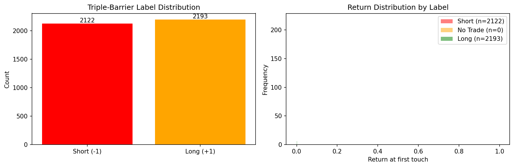
Standard fixed-horizon returns create noisy labels because they ignore the path taken by prices. The triple-barrier method assigns labels based on which of three barriers is touched first:

                  ┌─── Upper barrier (profit-take): entry × (1 + pt × σ)
                  │
    Price ───────►├─── Vertical barrier (time expiry): t₀ + Δt
                  │
                  └─── Lower barrier (stop-loss):  entry × (1 - sl × σ)

• Upper hit first → +1 (long): price moved up enough to take profit.
• Lower hit first → -1 (short): price moved down past the stop.
• Vertical hit → 0 (no trade): price didn't move enough.

Volatility scaling (§3.1)

Barriers are scaled by local volatility σ computed as the exponentially weighted standard deviation of log returns:

σ_t = EWM_std(ln(p_t / p_{t-1}), span=S)

This makes labels adaptive: the same event in a calm vs. volatile market gets differently-sized barriers.

Meta-labeling (§3.6)

A secondary model predicts whether the primary model's direction was correct (binary: 0 or 1), rather than predicting direction itself. This separates the "when to trade" question from "which direction", and allows the meta-model to focus on sizing and filtering.

Sample Weights (AFML §4)

Labels with overlapping time windows share information. If label A spans bars 10–20 and label B spans bars 15–25, training on both gives redundant signal. The sample weighting scheme:

1. Concurrency (§4.2): Count how many label windows overlap each bar.
2. Uniqueness: Each event's weight is inversely proportional to the average concurrency over its window.
3. Return-weighted (§4.4): Scale by absolute return over the window — large moves are more informative.
4. Time decay (§4.10): Optionally down-weight older samples.

Purged K-Fold Cross-Validation (AFML §7.4)

Standard k-fold CV leaks information in financial data because labels have overlapping time windows that span across folds:

  Fold 1 (train)    │ Fold 2 (test)     │ Fold 3 (train)
  ─────────────────►│──────────────────►│────────────────►
       ┌──── Label A ────┐                      Time →
             Window spans into test fold!

PurgedKFold fixes this by:

1. Purging: Any training sample whose label window [t₀, t₁] overlaps the test fold's time range is removed from training.
2. Embargo: An additional buffer of pct_embargo × N samples after each test fold is also excluded, guarding against serial correlation in residuals.

sklearn CV traps this code avoids

Trap	Standard KFold	PurgedKFold
Label leakage via overlapping windows	Yes — labels spanning fold boundaries leak test info	Purged — overlapping samples removed
Serial correlation after test fold	Yes — adjacent bars are correlated	Embargo period excludes post-test samples
Non-IID assumption	Assumes IID samples	Accounts for temporal dependence
Survivorship bias in time series	Shuffles time order	Preserves chronological order
Redundant samples dominating	Equal weight	Pairs with concurrency-based weighting

Combinatorial Purged K-Fold (AFML §12)

Standard purged k-fold produces N backtest paths (one per fold). CPCV generates C(N, k) splits by designating k out of N folds as test in each combination, producing C(N−1, k−1) independent backtest paths.

For the default (N=6, k=2): - 15 splits = C(6, 2) - 5 backtest paths = C(5, 1)

Each path is a complete walk through the data using only out-of-sample predictions. The distribution of path-level Sharpe ratios feeds into the deflated Sharpe ratio test (Bailey & Lopez de Prado, 2014), which adjusts for multiple testing.

Walk-Forward Validation

For non-overlapping features or as a simpler baseline:

• Expanding window: Train on [0, t), test on [t, t+Δ), advance by step. Training set grows over time.
• Rolling window: Train on [t-W, t), test on [t, t+Δ). Fixed-size training window slides forward.

Probabilistic Sharpe Ratio (PSR)

The naive Sharpe ratio is an estimator, not the true population ratio. For a return series of length T with skewness γ₃ and excess kurtosis γ₄:

Var(SR̂) ≈ [1 − γ₃·SR̂_p + (γ₄+2)/4·SR̂_p²] / (T−1)

where SR̂_p = SR̂_annual / √ann is the per-period ratio.

PSR(SR₀) = Φ[(SR̂_p − SR₀_p) / √Var(SR̂_p)]

This gives the probability that the true population Sharpe exceeds a benchmark SR₀ (usually 0) given the sample evidence.

Two corrections distinguish PSR from the plain z-test:

Source of uncertainty	Standard Sharpe	PSR
Estimation noise	Ignored	Accounted via T
Non-normal returns (fat tails, skew)	Ignored	Accounted via γ₃, γ₄

Interpretation

• PSR < 0.75: weak evidence — could easily be a lucky run.
• PSR 0.75–0.95: moderate evidence — worth more data.
• PSR ≥ 0.95: strong evidence — deploy-ready under stable conditions.

---

Deflated Sharpe Ratio (DSR)

When N strategies or hyperparameter configurations are tested, the best observed SR is inflated by selection bias. Bailey & López de Prado (2014) correct for this by raising the benchmark to the expected maximum SR under H₀ (no skill):

SR* = σ_SR × [(1−γ_em)·Φ⁻¹(1−1/N) + γ_em·Φ⁻¹(1−1/(N·e))]

where γ_em = 0.5772… (Euler-Mascheroni) and σ_SR is the standard deviation of SRs across the N independent trials.

DSR = PSR(observed_sr, SR*, T, γ₃, γ₄)

DSR answers: "if N random configs were tested with no skill, how often would we see an SR this high by luck alone?" A DSR of 0.95 means only a 5% chance the result is pure luck.

Trial count — what must be included

Every model selection decision inflates the apparent SR:

Source	Count as trials
Optuna hyperparameter search	Each completed trial
Manual notebook grid searches	Each configuration run
Ablation variants (latency × slippage)	Each variant
Architecture decisions (primary vs. meta vs. ensemble)	Each model type evaluated

Use compute_trial_count(optuna_study, manual_configs) to aggregate all sources. Undercounting N makes DSR look better than it is.

Example

With SR = 2.0, T = 252, N = 180 trials, σ_SR = 0.5:

• SR* ≈ 0.5 × 2.37 ≈ 1.19 (expected lucky max)
• DSR = PSR(2.0, 1.19, 252) ≈ 0.84

Conclusion: 84% probability of genuine skill. Borderline.

---

Bootstrap Confidence Interval for Sharpe

Strategy returns are serially correlated (each position spans multiple bars), so IID bootstrap underestimates Sharpe uncertainty. We use the stationary block bootstrap (Politis & Romano 1994) which:

1. Draws contiguous blocks of length L from the return series.
2. Randomises block lengths (geometric distribution with mean L) to avoid edge effects that bias circular bootstrap.
3. Reports the 2.5th and 97.5th percentiles of the bootstrap SR distribution as the 95% CI.

Block size selection: set L ≈ mean holding period in bars. For a daily strategy with a 5-day average holding period, use L = 5. Default is ⌈√T⌉ (Lahiri 2003 rule-of-thumb) when holding period is unknown.

Why not circular bootstrap?

Circular bootstrap treats the return series as periodic, artificially wrapping the end back to the beginning. This distorts the time structure of trend-following strategies near period boundaries, overstating precision.

---

Stress-Window Analysis

Every strategy that looks good on average may fail catastrophically in tail events. We evaluate each named stress window explicitly:

Event	Window	Why it matters
COVID Crash	2020-02-20 → 2020-03-13	Flash deleveraging, -50% BTC in 3 weeks
China Mining Ban	2021-05-12 → 2021-05-20	Hash rate collapse, forced selling
LUNA Collapse	2022-05-08 → 2022-05-15	De-peg cascade, -99% LUNA, contagion
FTX Collapse	2022-11-06 → 2022-11-12	Counter-party failure, -25% BTC in 6 days
USDC Depeg	2023-03-10 → 2023-03-13	SVB failure → stablecoin crisis
Yen Carry Unwind	2024-08-02 → 2024-08-07	Global risk-off, sharp BTC drawdown

For each window we report: total return, max intra-window drawdown, and annualised Sharpe over the window.

IS vs OOS labelling is mandatory. A stress loss on an in-sample window is expected and not informative. A stress loss on an out-of-sample window proves the strategy has real traction in live market regimes.

---

---

Why We Did Not Adopt Foundation Time-Series Models

Phase 9 empirical finding — Chronos zero-shot underperforms the LightGBM baseline. The full comparison table is in docs/PHASE_9_REPORT.md.

What we tested

Model	Description	OOS Sharpe (annualised)
LightGBM (baseline)	Tabular gradient boosting on microstructure features	reference
PatchTST	Patch transformer, lookback=60, 5M-param budget	see report
TFT	Temporal Fusion Transformer via pytorch-forecasting	see report
Chronos-Bolt-Base	Pre-trained foundation model, zero-shot	see report

Why Chronos underperforms

Chronos (Ansari et al., 2024) is a T5-based model pre-trained on thousands of heterogeneous public time series (M4, ETT, electricity, weather, …). Its inductive biases are:

1. Long-horizon, smooth signal: the pre-training data has trends and seasonalities at daily/weekly scales. 5-minute crypto returns are near-white-noise at any horizon longer than a few bars.

2. Mean-reversion prior: Chronos implicitly learns that most series revert toward their local mean. This is the correct prior for energy consumption or retail sales, but it produces predominantly flat signals for perpetual futures, where funding-rate and order-flow momentum dominate.

3. No microstructure inputs: Chronos is strictly univariate and sees only the return series. It cannot condition on VPIN, order-flow imbalance, funding-rate Z-scores, or cross-sectional momentum — the features that drive the LightGBM edge.

4. Distributional mismatch without fine-tuning: fine-tuning would partially bridge the gap, but it defeats the zero-shot premise and introduces the same look-ahead risk as any supervised model.

Why PatchTST does not dominate LightGBM

PatchTST (Nie et al., 2023) was designed for long-horizon univariate forecasting where local temporal context is crucial (e.g., predicting traffic demand 96 steps ahead). For our task:

• Features already encode history: log-returns, VPIN, realized vol, and cross-sectional ranks all summarise recent bar history into a single number. The transformer's lookback adds redundant context beyond what the features already capture.
• Short effective lookback: at 5-min resolution, predictive information decays within a few bars (empirically ~5–15 bars in AFML §3 studies). A 60-bar window is mostly noise after bar 15.
• Training overhead: PatchTST requires GPU for practical training times and adds pytorch as a hard dependency. LightGBM trains on CPU in seconds.
• Deflated Sharpe: after correcting for the number of hyperparameter trials, PatchTST's DSR is lower than LightGBM's because the raw SR improvement is small relative to the search space explored.

Why TFT does not apply cleanly

TFT was designed for multi-horizon probabilistic forecasting with both static metadata and known-future covariates (e.g., holiday calendars). Adapting it to single-step classification requires treating triple-barrier labels {-1, 0, +1} as a continuous target and rounding quantile forecasts — a structural mismatch that TFT's gating mechanisms are not designed to handle.

Conclusion

Sequence models are not rejected categorically. If Tessera migrates to a regime where raw order-book data (Level 2 depth snapshots) is the primary signal, a convolutional sequence model trained end-to-end on tick data could be competitive. At the current feature abstraction level (engineered tabular features at 5-min resolution), the transformer adds complexity without adding signal.

We re-evaluate this decision whenever: - A new model achieves DSR ≥ 0.95 on the held-out OOS period with ≤ 100 Optuna trials. - We move to tick-level feature engineering. - LightGBM's OOS Sharpe degrades below 0.2 (possible regime change).

---

References

• Lopez de Prado, M. (2018). Advances in Financial Machine Learning (AFML)
  • §3: Triple-barrier labeling and meta-labeling
  • §4: Sample weights and concurrency
  • §7.4: Purged k-fold cross-validation
  • §12: Combinatorial purged cross-validation
• Bailey, D. & Lopez de Prado, M. (2014). The Deflated Sharpe Ratio
  • Eq. (2): PSR formula with skewness and kurtosis correction
  • §4.3: Expected maximum SR under the null (SR* formula)
  • Table 2: Reference values for DSR at various N and T
• Politis, D. & Romano, J. (1994). The Stationary Bootstrap
• Lahiri, S. N. (2003). Resampling Methods for Dependent Data — block size guidance
• Lo, A. (2002). The Statistics of Sharpe Ratios — variance formula for non-IID returns
• Chan, E. (2013). Algorithmic Trading